Example 1

Choose a temperature and two different Mu values and start the simulation. Observe how the molecules are moving. Now click on the tab labeled "Number Density." You should see something that looks like this:

The red line here represents the blue molecules, while the blue line represents the white molecules. Each of these lines represents the number of molecules per unit volume. You can play around with the temperature and the different mu's to see what affect they have upon the number density profiles. At steady state, Fickian diffusion will be occurring and it can be noticed that both lines will be nearly linear around 1/2 of the total volume.

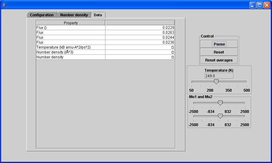
Another interesting feature of this simulation is the "Data" tab which appears at the start of the simulation. The "Data" tab will look something like this

The four fluxes seen here represent the flux of each species either moving into or out of one of the control volumes. Steady state is achieved when the amount of material going in, is the amount of material coming out. As seen here steady state is almost achieved.

When steady state is achieved, one can determine the diffusivity, using both the "Data" and "Number Density" tabs. To determine the diffusivity, use Fick's First Law with the measured flux and the nearly linear concentration gradient.